Abstract
Wavelet analysis methods are applied to find the main features of the human face. There exist methods of feature extraction based on banana wavelets that use 2-dimentional wavelets. We try to apply simple Gaussian Wavelets, more correctly called Vanishing Momenta Wavelet Family (VMWF). Applying that type of wavelets we use recently developed fast algorithms that allow to reach real-time preprocessing of the image.
Images
Face image is what is at the input of the system. The expected result of preprocessing stage is an image which contains only the significant features of the face. To avoid variations which present in the input image we will attempt to build an algorithm of averaging the details so that only main features remain.
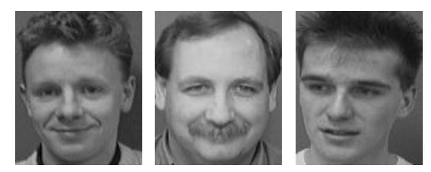
We restrict ourselves on processing of standard Windows bitmap format (*.bmp) pictures, but that of course does not restrict the possibility of working with any other presentation of an image. Our test images are of size approximately 100 on 100 pixels with 256 gray scale at every pixel. The Fig. 1 presents some examples of such images taken from the AT&T; Laboratories standard face image base.
Images are regarded as an array of numbers. The dimension of the array is defined by the width and the height of an image. The elements of an array are integer numbers within [0, 255] range. The usage of 256 colors bitmap format makes it easy to operate with the pixels without any additional work for the conversation of an image into the array of integer numbers. In our case one byte is one pixel.
Wavelet Instruments
Although the image is a two-dimensional structure we still use one-dimensional wavelet functions. One of the reasons of it is its speed comparing with the 2D-wavelets. To evaluate the wavelet image we use the fast method which we developed earlier.
The stage of extracting the features of the face from a unique image goes in two parallel branches — horizontal and vertical (that can be effectively used for parallel evaluations, and even more, the structure of each branch allows to split the task into subtasks, and the result will be updated after the subprocess is completed; no extra memory requests are needed). Both of the m use the same algorithm and therefore are easy in implementation — you just need to white a procedure for one of the branch and it is easy to modify the code for the other.
The whole process of feature extraction expects the se two substages and after doing that the results of the two branches are combined together so that a new image of the original size would appear. That final image is a monochrome one and contains a contour face.
The First Stage
The image is presented as an array of lines — horizontal ones in one branch and vertical in another. Each line is processed as a single one-dimensional signal of the length equal to the width (or the height) of an image. Every line is than undergone the wavelet transform. Let fi be the sequence of pixel values, the index i goes from 0 to N-1, where N is the width (or the height) of an image. The wavelet image of the line is defined by the following expression.
Here a and b stand for the dilation and shift parameters of the gaussian wavelet gn of order n. The shift b changes within the same range that index i does, that is [0, 255]. the choice of the scale a is a separate task. The wavelet is defined by the following general expression.
The normalization factor is
After doing that every horizontal and vertical line will be transformed into the wavelet space at the selected scale a. Red curve on the plot in the middle of Fig. 2 shows the highlighted line of the image shown at the top. The plot is given with notes marking different parts of the face. The wavelet image of the line is at the bottom plot. That image was evaluated using Gaussian wavelet of order 3 at the scale 1.5.
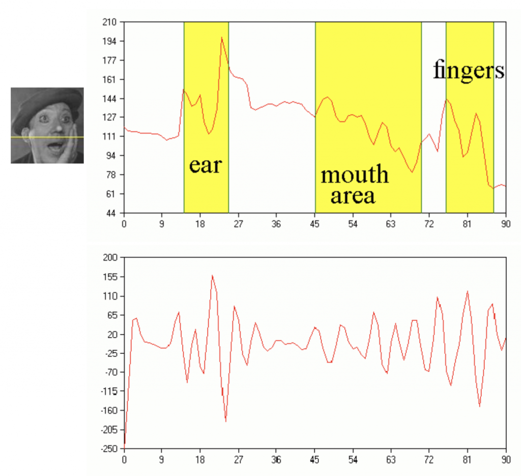
Fig. 2. The image, one line of it (that one which is marked on the picture) and its wavelet image.
The information contained in the wavelet image of the line includes both the face features and the noise. Before continuing we should denoise the wavelet image. The simplest way to do that is to exclude those parts of wavelet coefficients which are small in magnitude. You define the threshold and all the coefficients which are not so strong to overcome this barrier are set to zero. Being so simple the procedure suppresses the noise efficiently enough. The result of applying 20 % threshold to the wavelet coefficients shown on the Fig. 2 is depicted on the Fig. 3. Note that after denoising the area which corresponds to the cheek is a direct zero value line, showing that the re are no details on the face at that place.
This denoised wavelet image already reflects the most significant features on the face. But it still carries redundant information on the slopes of peaks. This redundancy can be easily excluded. The way of doing that is known as skeletizing of wavelet spectrum. To convert the wavelet image to the skeleton you just need to find all local maxima of the wavelet sequence. The result of this if presented on the Fig. 3 with blue ticks. Note that the skeleton can be stored into a boolean array, it does not include the information about the level of the signal at the maximum.
Thus after obtaining the skeleton we can start to build the new image. Pixels placed at the skeleton bones we mark black, other pixels are white. Applying the procedures described above we will obtain the picture which reflects the most significant features of the source image.
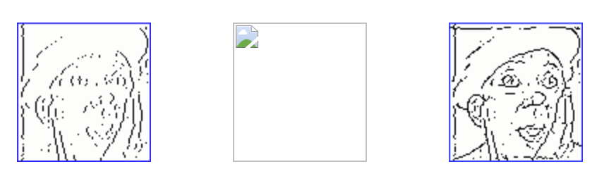
The result of converting an image from Fig. 2 is shown in Fig. 4. Left picture shows how the image will look after a branch of processing horizontal lines, the middle one is the result of another branch which extracts features from vertical lines. The sum of these both parts is on the right.
Further suppression of noise can be achieved by selecting the most «wide» local maxima in the wavelet coefficients sequences for each horizontal and vertical line. One need to define a depth value, i. e. the number of pixels that would appear before and after the maximum, all of them must be of lower level than the central pixel. By varying this additional parameter it is possible to slightly clear the skeleton from not significant elements which appeared because of the small sized details in the image. But if you will try to find too «deep» maxima the result will be opposite to what was expected to see. Several skeletons on Fig. 5 show the influence of the depth parameter.
Wavelet Order and Scale
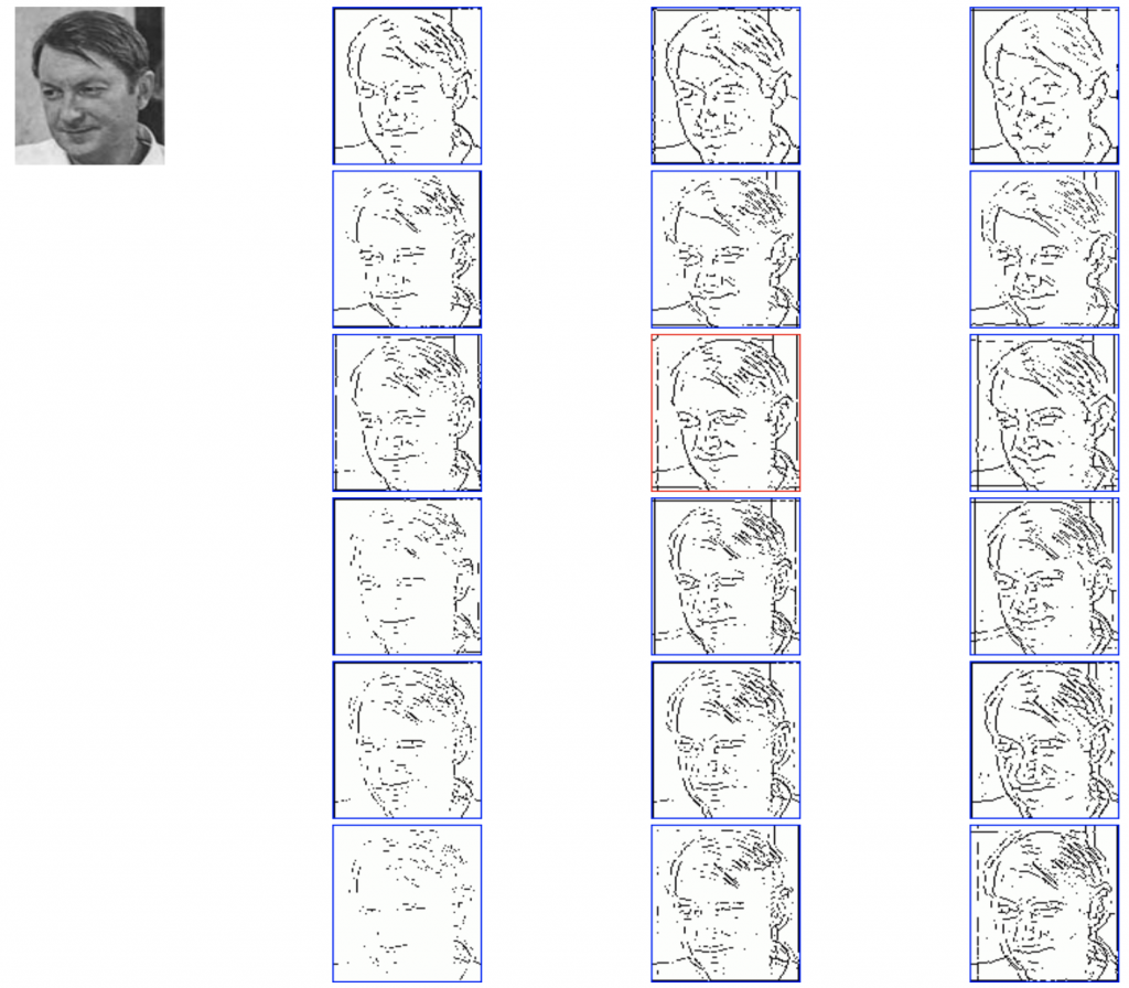
To convert an image into its skeleton one needs to choose the order of the wavelet and the scale at which to perform the transform. Our experiments with various wavelets from WMVF at different scales clearly shows that the best choice is Gaussian wavelet of order 3 at scales of 1.5 trough 2. No doubt this scale range is only appropriate if the image size does not differ much from selected by us, that is 100 on 100 pixels. Fig. 6. presents several images obtained with wavelets of orders 1 through 6 at scales 1, 1.5 and 2. Note the appearance of double contour lines with the higher order wavelets. The threshold everywhere is 20 % and the depth rate is 3.
Averaging Face Skeletons
Further information describes my attempt to use several images of one face to create averaged bitmap. Results show that if you wish to use skeletized images in face recognition systems you should average vector-based features rather than bitmaps.
Coarsening
Scan through all the pixels of the image, if there are enough (defined by an Area Threshold) neighbours, the result is a black pixel on the new image.
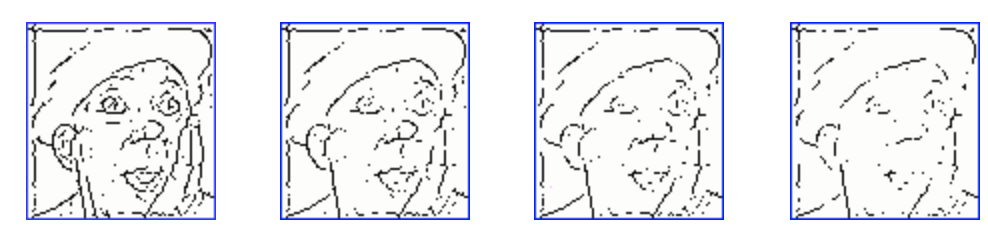
Examples of coarsening
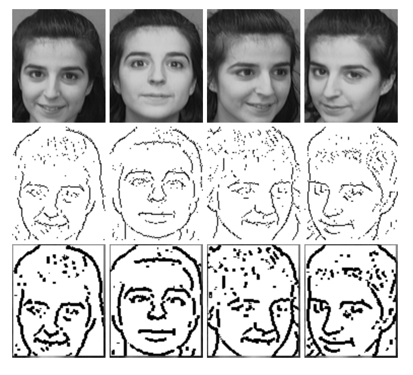
Four of 10 source images (top), their skeletons (middle) and coarsen skeletons (bottom).
Averaging
After applying the coarsening procedure to all the images, nearly the same procedure is applied to images, obtained during that stage. Pixel neighbour this time is the pixel with the same position placed on another image.
The most difficult for averaging are set of images where faces are not frontal only. The goal is to get the frontal average image.
Examples of averaging
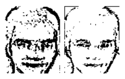
Averaged skeletized image of 10 images of the face above. The head rotation caused an effect of photographing the moving objects (left image). An attempt of decreasing the influence of head rotation was made (by straightening the Depth parameter at the stage of skeletizing and the Planes Threshold at the averaging stage.
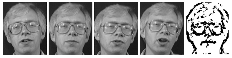
One more example. This time the resulting image is rather good, no head rotation influence is visible although head angles are clearly seen on the source.
One thought on “Face Image Preprocessing Based on Wavelets”